Using The Keyword Planner For SEO

Using The Google Adwords Keyword Planner To Plan An SEO Strategy

In my last blog post which was featured on SEMrush’s Blog,  I discussed how to use Google Analytics and Excel to find and organize the highest quality keywords from a large data sample. I explained how to use a few excel formulas to simplify your data organization and ultimately end up with a really thorough keyword strategy for SEO, PPC or both. Today I will be taking this process one step further and show you how to use Google Adwords’ keyword planner to get keyword search volumes and integrate them into your Analytics + Adwords data. I will also show you how to use charts in Excel to help you sort out inferior keywords.

Pivot Tables and The Vlookup Function

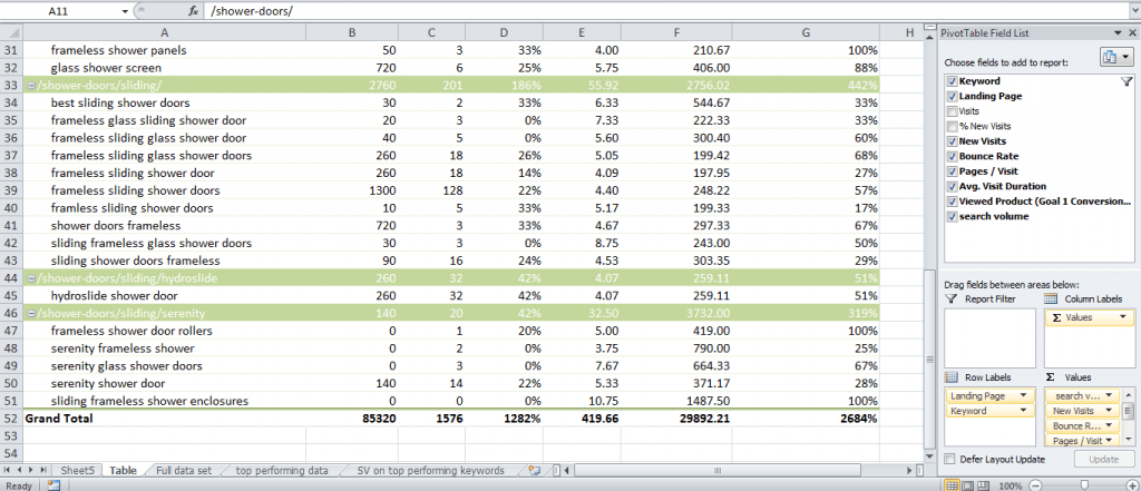
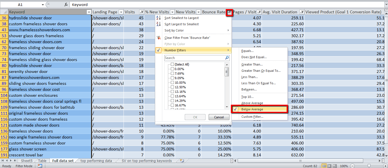
If you didn’t read the last blog post on this subject please do so before continuing to read this post as it will not make sense. We will begin where I left off in my last blog post. You should have an excel spread sheet organized in a pivot table as shown to the left (click to enlarge). Keywords should be listed underneath their designated landing pages in column A.  The columns next to column A contain various metrics from Analytics like number of visits for that keyword and other common metrics like time on site, average visitor duration and bounce rate. We will now add a new column, “Search Volume”. In order to do this you will need to go back into Google Analytics and export the same data into Excel that you used to create the pivot table. Once this data is in Excel click on “Insert” and then click on “Table”. The entire spreadsheet will turn blue and you will notice drop down arrows have appeared next to each column heading. Now you can filter out keywords based on their metrics performance. Since we are dealing with large data samples containing thousands of keywords I like to remove some of the obvious poor performing keywords right of the bat . We can do this by placing filters on metrics that are most relevant for predicting the performance of a keyword. These metrics include “pages/visits”, “Bounce Rate”, and “Avg. Visit Duration”. Click on the dropdown arrow next to “pages/visits” scroll down to “number filters” and click on “greater than”. Now you can enter in the minimum number of pages viewed that that keyword produced. For the first filter I usually choose 2. Now that all keywords that produced less than 2 page views are gone we will now place a filter on “Bounce Rate”. First, we need to make this column a percentage. Highlight the column and under “Home” on the Excel navigation you will find a % button. Once you have changed that column to percent click on the drop down arrow then “number filters” and finally “Below average” this will remove all the keywords with above average bounce rates. Next we filter “Avg. Visit Duration”. For this metric we click on the “Above Average” filter to remove all the keywords that brought visitors who spent below average time on your site. Now that many of the poor performing keywords have been removed from our chart we can work on getting  search volumes. Below is a snapshot of the excel table I have been working, as you can see the option to filter columns is fairly easy to use. In the screen shot, I show how to filter out keywords that have an above average bounce rate.

Getting Search Volumes From Key Word Planner

Now that we have a ton of keyword ideas and the metrics which tell us how visitors performed when they found your site via these keywords, wouldn’t it help to know which of these top performing keywords have a high search volume? Lets go ahead and do that. Login to your Google Adwords account and click on “Tools and Analysis” then “keyword planner”. Now select “Get search volume for a list of keywords or group them into ad groups”. A box will appear where you will copy and paste all the keywords from your Excel chart, then click “Get search volume”. Click on the tab “keyword ideas” and then click “Download”. You now have two Excel books open. One with your chart and another with your search volumes. Because we want to combine this data you will need to copy all the keywords and their search volumes and paste them into the Excel book with your chart.

Vlookup Function

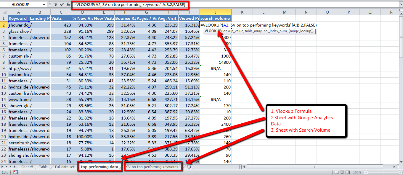
So now that you have they keyword search volume, you will need to copy the two columns (keyword column and search volume column) and put them in the same work book that you are working on but in a separate sheet. With your chart and a spreadsheet with all your keyword search volumes we will use the most efficient method for combining them, a vlookup function. In your original sheet with the data from Analytics, add a column all the way to the right for search volume. In the first cell, name the column “search volume” and in the cell just below that we will call the “vlookup” function which is:

“=vlookup(lookup_value, table_array, col_index_num, [range_lookup])”   

You will need to do a few things to get this working right but once you do its a game changer. You simply have to call the function by entering “=vlookup()”, but in the parenthesis you have to specify a few things. First you will have to tell the function where to search for keywords, so you should probably enter “a2” because that is where the first keyword appears. After entering “a2” you must separate the next variable with a comma so you should have at this point “=vlookup,a2,”, next we need to specify where the function is supposed to aggregate the data from so you should click on the first keyword on your new sheet from the keyword planner tool which is on a separate sheet. Notice that when you click on the new sheet, if you are editing the cell with the formula, excel will add the name of the sheet (in a set of single quotes followed by an exclamation mark) in the function after the comma that you last entered. So now you will have something like this =VLOOKUP(A2,’SV on top performing keywords’!. We are just about done now. The last thing we need to do is specify the location of the keywords and the location of the corresponding search volume which you are trying to aggregate. To do this, simply add the letter of the columns separated by a colon. Ideally, you should have your keywords in column A and your search volume in column B which would mean that your function should now look like this: =VLOOKUP(A2,’SV on top performing keywords’!.

Last but not least, you will need to add the following “2,false”. I won’t go into why this is needed because it is more of a programming thing and you don’t need to worry about why this is added. If you really want to know, feel free to leave a comment. Below are the explanations as to what you are calling in the function.

• lookup_value  – The value to search in the first column of the table or range. The lookup_value can be a value or a reference. If the value you supply for the lookup_value is smaller than the smallest value in the first column of the table_array argument, VLOOKUP returns the #N/A error value.
• table_array  – The range of cells that contains the data. You can use a reference to a range (for example, A2:D8), or a range name. The values in the first column of table_array are the values searched by lookup_value. These values can be text, numbers, or logical values. Uppercase and lowercase text are equivalent.
• col_index_num  –  The column number in the table_array argument from which the matching value must be returned. A col_index_num argument of 1 returns the value in the first column in table_array; acol_index_num of 2 returns the value in the second column in table_array, and so on.
• range_lookup    Optional. A logical value that specifies whether you want VLOOKUP to find an exact match or an approximate match. If range_lookup is either TRUE or is omitted, an exact or approximate match is returned. If an exact match is not found, the next largest value that is less than lookup_value is returned.

Below is a screen shot of the sheet I am using as an example, hopefully this will work for the visual learners.

Now that you have the formula in one cell you can drag that formula down for the rest of the column. We now need to use are filters again and in order to do this we need to copy and paste this data onto another page and insert another chart. Click on the “greater than or equal to” filter and enter the number 1. Now that we have removed all the keywords that have no search volume we need to take a look at how many keywords we have left. If you still have over 300 I would go back into filters for the three metrics I mentioned earlier and get a little more picky. Once you are left with approximately 100-200 solid keywords you can insert a pivot table to make the data easier to read.

You are finally left with a very easy to understand spreadsheet that contains the cream of the crop; a batch of very popular keywords that will consistently drive quality traffic to your website. As a PPC management company owner, I strive to use these types of techniques for our clients whether its an SEO or PPC campaign. I hope you find this useful! Thanks for Reading!

About The Author

Jason Hawkins / http://www.themiamiseocompany.com

Jason Hawkins is the CEO & Co-Founder of The Miami SEO Company. He has over ten years of experience in search engine optimization, conversion rate optimization and lead generation. His core responsibilities include identifying ways to increase value of services rendered, training staff on advanced SEO topics, and A/B testing internal processes to consistently improve client return on investment.